Chapter 6: Graphs and Trees
Section 6.3 Decision Trees
We learn decision trees when studying the lower bound of searching and sorting because they provide a visual and theoretical framework to understand the minimum number of comparisons required to solve these problems.
Decision Tree
The concept of using a decision tree for sorting follows a similar structure as with searching algorithms, but instead of comparing a target value to items in a list, you are comparing pairs of items within the list to determine their order.A decision tree is a tree in which the internal nodes represent actions, the arcs represent outcomes of an action and the leaves represent final outcomes.
Sometimes useful information can be obtained by using a decision tree to represent the activities of a real algorithm; actions that the algorithm performs take place at internal nodes, the children of an internal node represent the next action taken, based on the outcome of the previous action, and the leaves represent some sort of circumstance that can be inferred upon algorithm termination.
Decision Tree in Sorting Algorithms
In sorting algorithms, a decision tree is a theoretical model that helps us understand the minimum number of comparisons needed to sort a list using comparison-based sorting algorithms like merge sort, quick sort, or bubble sort.In the context of sorting algorithms, a decision tree is a conceptual tool used to represent all possible comparisons that a comparison-based sorting algorithm might make to sort a given set of elements. The tree helps visualize the sorting process by showing the sequence of comparisons, with each path from the root to a leaf representing a possible outcome (sorted order).
Sorting
Decision trees can also model algorithms that sort a list of items by a sequence of comparisons between two items from the list. The internal nodes of such a decision tree are labeled L[i]:L[j] to indicate a comparison of list item i to list item j. To simplify our discussion, let's assume that the list does not contain duplicate items. Then the outcome of such a comparison is either L[i] < L[j] or L[i]> L[j]. If L[i] < L[j], the algorithm proceeds to the comparison indicated at the left child of this node; if L[i]> L[j], the algorithm proceeds to the right child. If no child exists, the algorithm terminates because the sorted order has been determined. The tree is a binary tree, and the leaves represent the final outcomes, that is, the various sorted orders.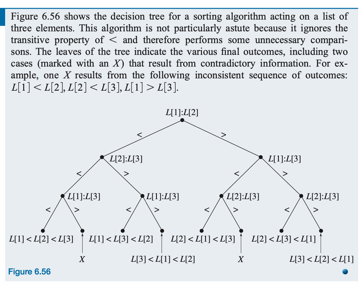
A decision tree models every possible sequence of comparisons that could happen while sorting n elements.
- ♣ Each node in the tree represents a comparison (e.g., "Is L[1] > L[2]?").
- ♣ Each branch shows the result of the comparison (yes/no or true/false).
- ♣ Each leaf node represents one possible sorted order of the array.
Bubble Sorting Demo
| Case | Time Complexity | Explanation |
|---|---|---|
| Best Case | O(n2) | Array is already sorted; n(n - 1)/2 comparisons, 0 swaps. |
| Average Case | O(n2) | Random order; n(n - 1)/2 comparisons. |
| Worst Case | O(n2) | Array is in reverse order; maximum number of swaps and comparisons. |
Understanding \( \frac{n\times(n-1)}{2} \) comparisons
- ♣ On the 1st pass, it does n−1 comparisons
- ♣ On the 2nd pass, it does n−2 comparisons
- ♣ On the 3rd pass, it does n−3 comparisons
- \(\dots\)
- ♣ On the (n−1)th pass, it does 1 comparison
- ♣ So the total number of comparisons is: \(1 + 2 + \dots + (n-1) = \frac{n\times(n-1)}{2} \)
Lower Bound for Sorting
Theorem: On the Lower Bound for SortingAny algorithm that sorts an n-element list by comparing paris of items from the list must do at least ⌈\(log_2 n!\)⌉ comparisons in the worst case.
This theorem gives us a lower bound on the number of comparisons required in the worst case for any algorithm that uses comparisons to solve the sorting problem.
(Lower bound means no algorithm can get faster than this no matter what, so if an algorithm actually does this, then it is optimal for worst case scenario)
Note:
(1) ⌈⌉ means ceiling. The ceiling is the smallest integer that is greater than or equal to the number inside the ceiling signs.
For example:
⌈2.9⌉=3
⌈2.4⌉=3
⌈2⌉=2
(2) log is actually base 2 even though they didn't put the base in the statement of the theorem.It is stated elsewhere.
(3) \(log_2x = y\) means \(2^y=x\) so \(log_2 n\) means that we want the exponent we would need to put on 2 in order to get n.
(4) Example 1:
Any algorithm that solves the sorting problem for a 3-element list by comparing Paris of items from the list must do at least __________ comparisons in the worst case.
Solution: ⌈\(log_2 3!\) ⌉ = ⌈ \(log_2 6\)⌉ = ⌈2.???⌉ = 3
How did we get this? The table below has powers of 2 up to \(2^{13}\), and if we want to know the value of x when \(2^x=6\) (because log 6 = x means \(2^x=6\)), then looking in the table (4 < 6 < 8), so x must between 2 and 3. Because of the ceiling, ⌈2.???⌉ = 3, we don't have to know the value of the ????.
| x | \(2^x\) |
|---|---|
| 1 | 2 |
| 2 | 4 |
| 3 | 8 |
| 4 | 16 |
| 5 | 32 |
| 6 | 64 |
| 7 | 128 |
| 8 | 256 |
| 9 | 512 |
| 10 | 1024 |
| 11 | 2048 |
| 12 | 4096 |
| 13 | 8192 |
(5) Example 2:
Any algorithm that solves the sorting problem for a 5-element list by comparing paris of items from the list must do at least __________ comparisons in the worst case.
Solution: ⌈\(log_2 5!\) ⌉ = ⌈ \(log_2 120\)⌉ = ⌈6.???⌉ = 7
(6) Example 3:
Any algorithm that solves the sorting problem for a 7-element list by comparing paris of items from the list must do at least __________ comparisons in the worst case.
Solution: ⌈\(log_2 7!\) ⌉ = ⌈ \(log_2 5040\)⌉ = ⌈12.???⌉ = 13