Chapter 6: Graphs and Trees

Section 6.1 Graphs and Their Representations

Computer Representation of Graphs

We have said that the major advantage of a graph is its visual representation of information. What if we want to store a graph in digital form? Although it is possible to store a digital image of a graph, it takes a lot of space. Furthermore, such an image remains but a picture --- the data it represents can't be manipulated in any way. What we need to store these essential data that are part of the definition of a graph -- what the nodes are and which nodes have connecting arcs. From this information, a visual representation could be reconstructed if desired. The usual computer representations of a graph involve one of two data structures, either an adjacency matrix or an adjacency list.

Adjacent Matrix

An adjacency matrix is a 2D array where rows and columns represent vertices (nodes), and each cell (i, j) indicates whether there is an edge between vertex i and vertex j.

An adjacency matrix is a square matrix used to represent a graph in mathematics and computer science. For a graph with $n$ vertices, the adjacency matrix is an $n \times n$ matrix where each element indicates whether pairs of vertices are adjacent or not.

Suppose a graph as $n$ nodes, numbered $n_1,n_2,\dots,n_n$. This numbering imposes an arbitrary ordering on the set of nodes. Having ordered the nodes, we can form an $n \times n$ matrix where entry $(i,j)$ is the number of arcs between nodes $n_i$ and $n_j$. This matrix is called the adjacency matrix A of the graph with respect to this ordering. Thus: $$ a_{ij} = p, \text{where there are p arcs between } n_i \text{ and } n_j $$
Here’s how it works:

If there is an edge between vertex i and vertex j, the matrix entry at position (i,j) will be 1 (or some positive value for weighted graphs).
If there is no edge between vertex i and vertex j, the matrix entry at position (i,j) will be 0.

Example 1: Undirected Graph

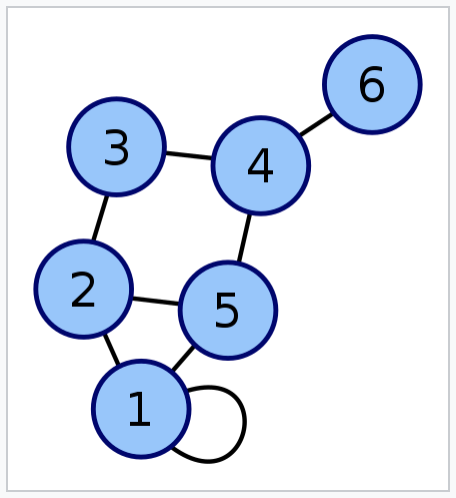
The adjacency matrix for the graph in Figure 1 with respect to the ordering 1,2,3,4,5,6 is a $6 \times 6$ matrix. Entry (1,1) is a 1 due to the loop at the node. All other elements on the main diagnola are 0. Entry (2,1) (second row, first column) is a 1 because there is one arc between node 2 and node 1, which also means that entry (1,2) is a 1.
$$ \begin{pmatrix} 1 & 1 & 0 & 0 & 1 & 0 \\ 1 & 0 & 1 & 0 & 1 & 0 \\ 0 & 1 & 0 & 1 & 0 & 0 \\ 0 & 0 & 1 & 0 & 1 & 1 \\ 1 & 1 & 0 & 1 & 0 & 0 \\ 0 & 0 & 0 & 1 & 0 & 0 \\ \end{pmatrix} $$

Figure 1 The adjacency matrix in Figure 1 is symmetric, which will be true for the adjacency matrix of any undirected graph -- if there are p arcs between $n_i$ and $n_j$, there are certainly p arcs between $n_j$ and $n_i$.They the symmetry of the matrix means that only elements on or below the main diagonal need to be stored. Therefore, all the information contained in the graph in Figure 1 is contained in the "lower triangular" array. For undirected graphs, the adjacency matrix is symmetric.

adjacencyMatrix.cpp

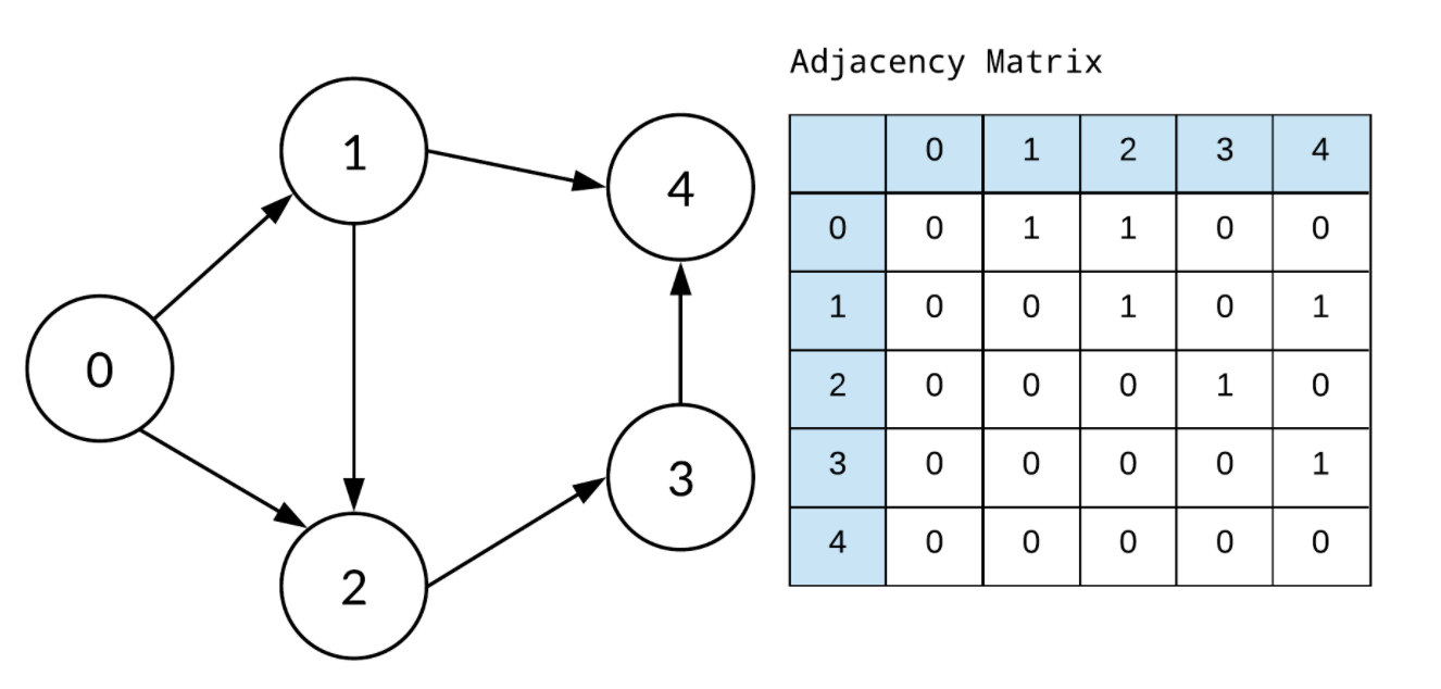
Example 2: Directed Graph

An adjacency matrix for a directed graph will not necessarily be symmetric, because an arc from $n_i$ to $n_j$ does not imply an arc from $n_j$ and $n_i$. See the example in Figure 2:

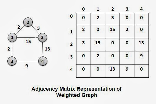
Figure 2 Example 3: Weighted Undirected Graph

In a simple weighted graph, the entries in the adjacency matrix can indicate the weight of an arc by the appropriate number rather than just indicating the presence of an arc by the number 1.

Figure 3

Adjacent Matrix Advantages vs Disadvantages

✅ Advantages	❌ Disadvantages
✅ Fast edge lookup: Checking if an edge exists between two nodes is O(1).	❌ High space complexity: Requires O(V²) memory, even if the graph has few edges.
✅ Simple implementation: Easy to implement using a 2D array.	❌ Inefficient for sparse graphs: Wastes space when many entries are 0 (no edge).

Practice

Please find the adjacency matrix: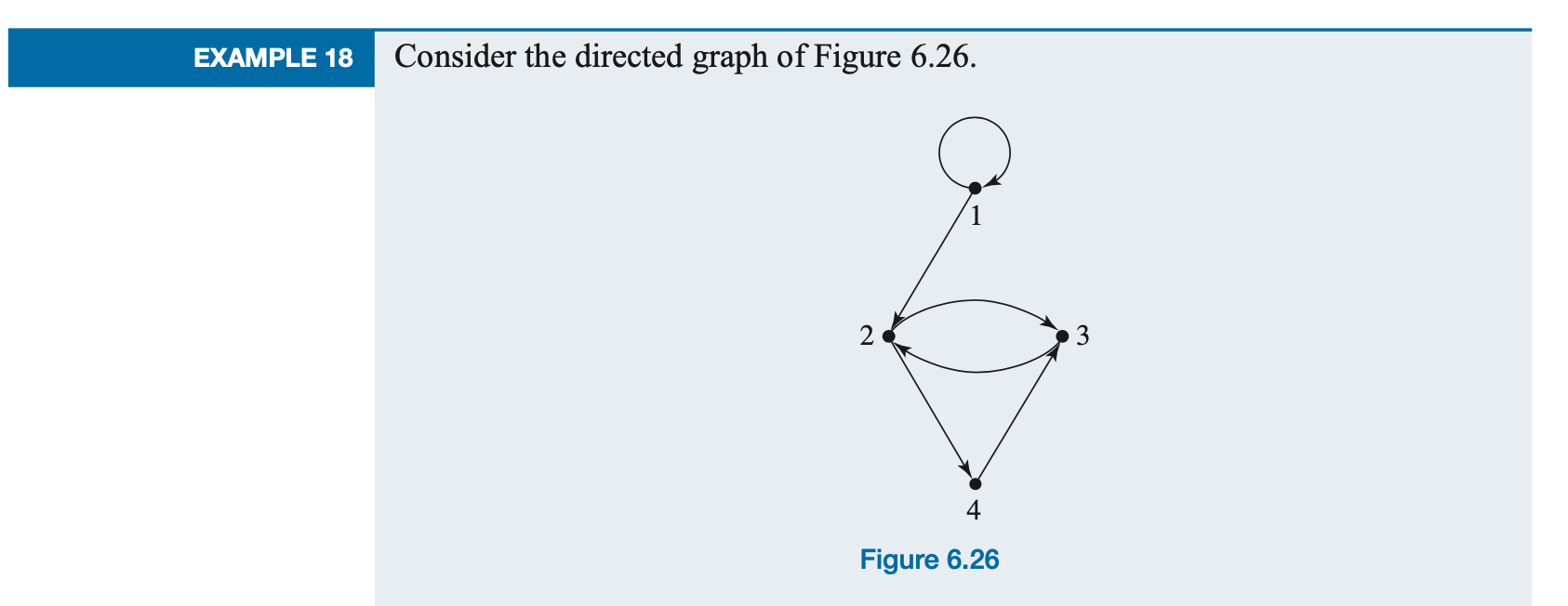

Real-Life Application of Adjacency Matrix: Flight Route System

Imagine we are building a flight booking system for an airline.

♣ The cities New York (NYC), Los Angeles (LAX), Chicago (ORD), and Dallas (DFW) are represented as nodes.
♣ A direct flight between two cities is represented as an edge.
♣ If a flight exists between two cities, we mark it as 1; otherwise, it's 0.

Step 1: Representing Flight Routes Using an Adjacency Matrix

♣ If there is a flight between city[i] and city[j], then matrix[i][j] = 1, otherwise 0.
♣ Since flights are bidirectional (undirected graph), the matrix is symmetric.

City	NYC	LAX	ORD	DFW
NYC	0	1	1	0
LAX	1	0	1	0
ORD	1	1	0	1
DFW	0	0	1	0

Step 2: Implementing the Adjacency Matrix in C++

adjacencyMatrix.cpp

Reference

saylor academy