Chapter 6: Graphs and Trees

Section 6.1 Graphs and Their Representations

Computer Representation of Graphs

We have said that the major advantange of a graph is its visual representation of information. What if we want to store a graph in digital form? Although it is possible to store a digital image of a graph, it takes a lot of sapce. Furthermore, such an image remains but a picture --- the data it represents can't be manipulated in any way. What we need to store are these essential data that are part of the definition of a graph -- what the nodes are and which nodes have connecting arcs. From this information a visual representation could be reconstructed if desired. The usual computer representations of a graph invovle one of two data structures, either an adjacency matrix or an adjacency list.

Many graphs, far from being complete graphs, have relatively few arcs. Such graphs have sparse adjacency matrices; that is, the adjacency matrices contain many zeros. A graph with relatively few arcs can be represented more efficiently by stor- ing only the nonzero entries of the adjacency matrix. This representation consists of a list for each node of all the nodes adjacent to it. Pointers are used to get us from one item in the list to the next. Such an arrangement is called a linked list. There is an array of n pointers, one for each node, to get each list started. This adjacency list representation, although it requires extra storage for the pointers, may still be more efficient than an adjacency matrix.

Adjacent List

An adjacency list is a collection of linked lists, where each node stores a list of adjacent vertices (i.e., the nodes it's connected to).

Many graphs, far from being complete graphs, have relatively few arcs. Such graphs have sparse adjacency matrices; that is, the adjacency matrices contain many zeros.
A graph with relatively few arcs can be represented more efficiently by storing only the nonzero entries of the adjacency matrix. This representation consists of a list for each node of all the nodes adjacent to it. Pointers are used to get us from one item in the list to the next. Such an arrangement is called a linked list . There is an array of n pointers, one for each node, to get each list started. This adjacency list representation, although it requires extra storage for the pointers, may still be more efficient than an adjacency matrix.

Example 1: Undirected Graph

The following figure shows two representations of an undirected graph. (a) An undirected graph G with 5 vertices and 7 edges. (b) An adjacency-list representation of G. (c) The adjacency-matrix representation of G.

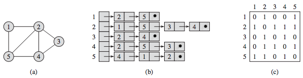
Figure 1 The adjacency list for the graph in Figure 1 contains a five-element array of pointers, one for each node. The pointer for each node points to an adjacent node, which points to another adjacent node, and so forth. In the figure the dot indicates a null pointer, meaning that there is nothing more to be pointed to or that the end of the list has been reached. We have dealt with parallel arcs by listing a given node more than once on the adjaceny list for \(n_i\) if there is more than one arc between \(n_i\) and that node.
Note that the arrow in list 3 from the 2 node to the 4 node does not mean that there is an arc from node 2 to node 4; all the elements in the node 3 list are adjacent to node 3, not necessarily to each other.

Example 2: Directed Graph

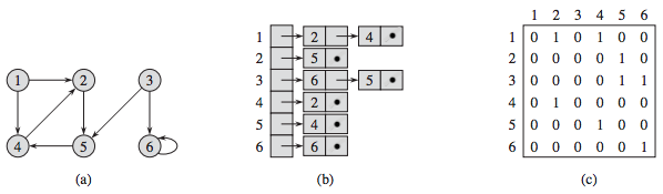
The following figure shows two representations of a directed graph. (a) A directed graph G with 6 vertices and 8 edges. (b) An adjacency-list representation of G. (c) The adjacency-matrix representation of G.

Figure 2 Reference

Example 3: Weighted Directed Graph

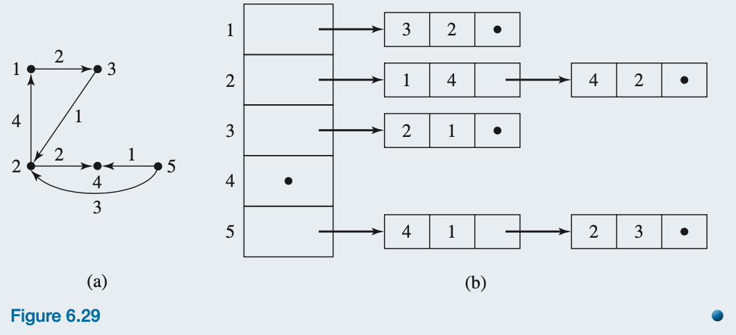
Figure 6.29a shows a weighted directed graph. The adjacency list representation for this graph is shown in Figure 6.29b. For each record in the list, the first data item is the node, the second is the weight of the arc to that node, and the third is the pointer. Note that entry 4 in the array of startup pointers is null because there are no arcs that begin at node 4.

Adjacent List Advantages vs Disadvantages

✅ Advantages	❌ Disadvantages
✅ Space-efficient: Uses only O(V + E) memory, ideal for sparse graphs.	❌ Slower edge lookup: Checking if an edge exists may take O(V) in the worst case.
✅ Efficient for iterating neighbors: Finding all edges of a node is O(degree of node), which is faster than scanning a whole matrix.

Practice

Please find the adjacency list: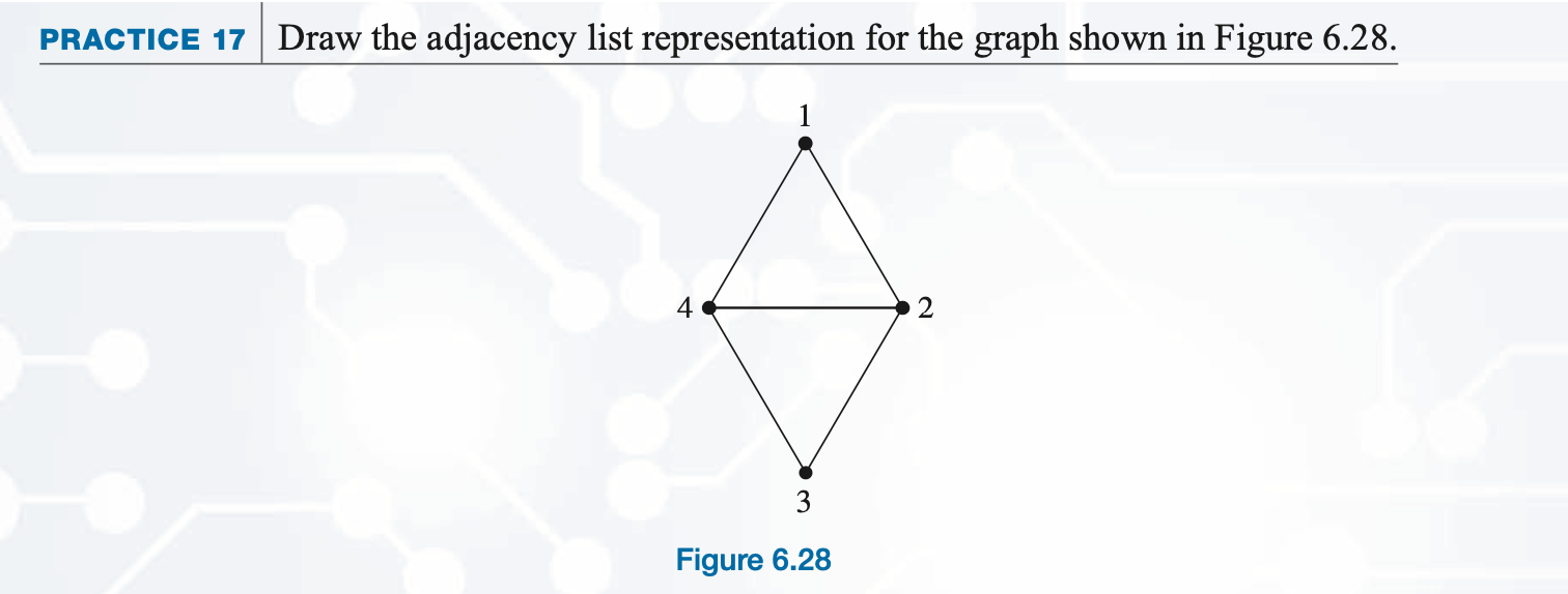

Real-Life Application of Adjacency List: Social Network Friendships

A common real-world use case for an adjacency list is in social networks, such as Facebook, LinkedIn, or Twitter. In these platforms:

Users are represented as nodes (vertices).
Friendships (or follow relationships) are represented as edges.
Since each user only connects to a small subset of all users, storing relationships in an adjacency matrix (which takes O(V²) space) is inefficient.
An adjacency list is the preferred approach since it scales well with millions of users.
Design a social network system where:

Users can connect as friends.
The system can display a user's friends.
The system can suggest new friends (friends of friends).

C++ Implementation: Social Network Graph Using Adjacency List

SocialNetwork.h
SocialNetwork.cpp
main.cpp

Reference

saylor academy